First version of my robot was made out of Lego mindstorm and controlled by a Raspberry Pi 1. Lego Mindstorm is amazing and I really wish it existed when I was a kid. So I took the motors from the Lego kit and used a L293 to drive them from the Rpi.
A few hours on figuring out how to put everything together in Lego and I got the “prototype” that you can see here in action following a line using the raspberry pi camera and openCV.
Eventually, 3D printers became a thing and the price decreased. It is still a little bit expensive but it is such a nice tool that I bought a kit to build a Prusa i3 rework. It is a fork of the popular prusa I3 which is one the most popular open hardware 3D printer. I liked the idea that many part of the printer was 3D Printed and it could print itself. Kit is delivered with a good assembly instructions manual, it’s a nice building game which is not too difficult but takes a few hours.
This is it in action printing it’s first part: a cube. I could just stay for hours starring at that thing building something layer after layer … it’s some kind of magic (but much slower).
Difficult part with such 3D printer is having a good calibration. A commercial 3D printer comes already calibrated so it can be used directly out of the box but it is not the case for DIY printers. Critical part is getting the first layer correctly. As it is very close to the bed, if the extruder is too close it can touch it (it would be bad) but if it is too far away the material won’t stick and every other layers will be messy. The complete configuration and calibration process, could probably be the subject of a complete post. Anyway, after many attempts and a few customization (bed height sensor, additional cooling fan), I have now a fully armed and operational battle station 3D printer. It’s time to make the Yapibot.
There is already a lot of robot design available on 3d model sharing site but I wanted to learn as much as possible so I decided to design also the parts. I did not touch any CAD software since high school, I had to start from scratch and learn everything. I always favour open source software when available and FreeCAD was an obvious choice. It’s open source and available for linux, windows and MAC. It took me a little bit of time to sort it out, but once you get the work flow, it does the job well. Draw a 2D sketch, add the constrains (dimensions) and extrude or create a pocket. Repeat on the next face… and so on until your part is done. Many tutorials are available to get you started. As I kept the part design as simple as possible using only basic shapes it went reasonably well. Only issue I faced, other than the few bugs from time to time, has been to do modification. As the building of a part is sequential and each sketch depends on each other, sometime a small modification of a dimension on a sketch will breaks the complete part, requiring to redo the complete design.
It’s probably not the best approach but I couldn’t figure the whole thing all together so I decided to go for modularity by making a “base” where I could just screw the other parts. This makes the design of each individual part much easier and easy to replace. Good thing about having your own 3D printer is that It’s easy to redo a part if it needs to be. As I’m exclusively using PLA as printing material (my 3D printer supports ABS but It’s not renewable, and emits toxic vapour while printing) I don’t have any remorse in trashing a part and re printing it.
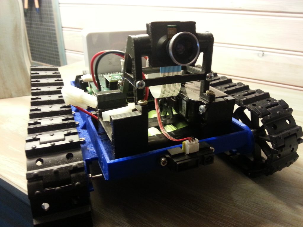
I kept to the caterpillar because it makes the mechanics easy to design, it can run on a great variety of surface and provide a good agility to the robot. However it is not the most precise method because by design it is drifting when turning. Motors can be found here. I choose DC motors because the command electronic is simple than stepper motors. they have a low max current so two motors can be driven by a single L293D without external components or heat-sink. Finally they have built in encoder that can be used to make a closed loop control and to measure the distance moved by the robot. I choose the 1:53 gear ratio because I was a little bit concerned about the motor capabilities but 1:19 would have been better in the end. Motors are powered by a specific batteries pack made of five 1.2V 2000mA/h AAA elements.
Tracks are from makeblock: http://www.makeblock.com/track-with-track-axle-40-pack (I used one and half pack). That’s the only mechanical part not printed. Printed parts are unfortunately too slippery for this usage.
Here is the CAD result showing only the printed part.
And here are the files :FreeCAD Files.
Printing a part can takes several hours depending on the number of layers.
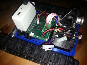
Work in progress ….
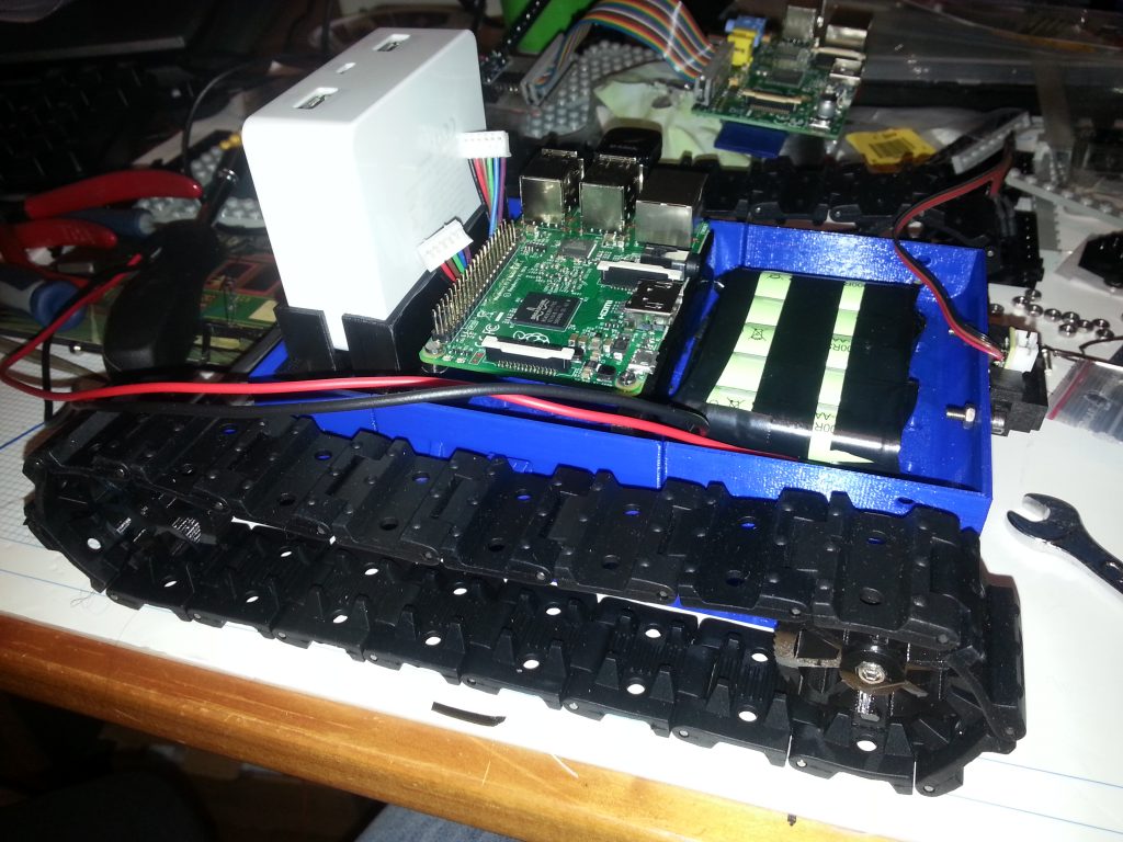
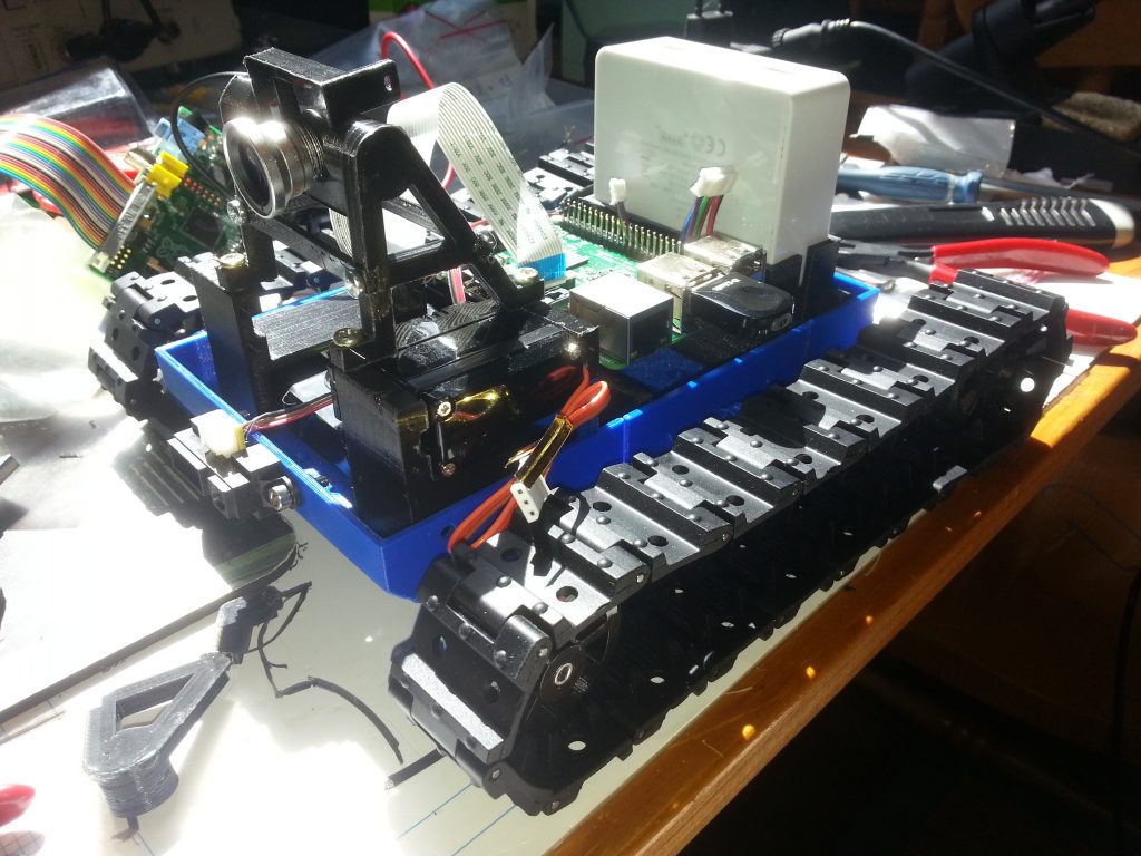
… and done (for the moment).
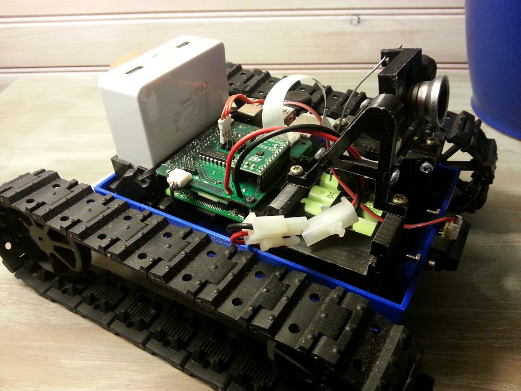
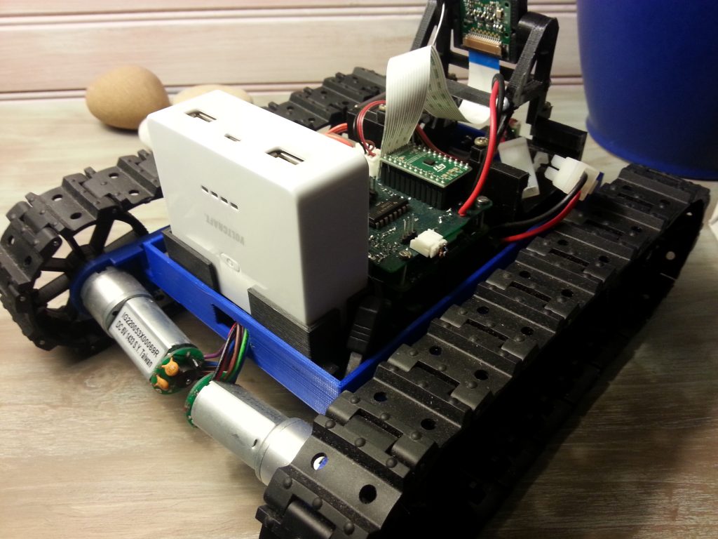
There is still an issue that I didn’t tackled yet. Motors fixing is not rigid enough and flex too much due to the motor weight and caterpillar tension. It’s not a big issue for the moment, but it might be if more precision is needed.
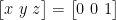

 ,
,  , and
, and  are the measurement done on the according axes,
  is the scalling error and
  is the offset error.


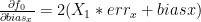
 it can be shown that
  can be left multiply by the inverse of its jacobian matrix.


 ,
,  ,
,  ,
,  ,
,  , and
, and  .
. on
on  we get:


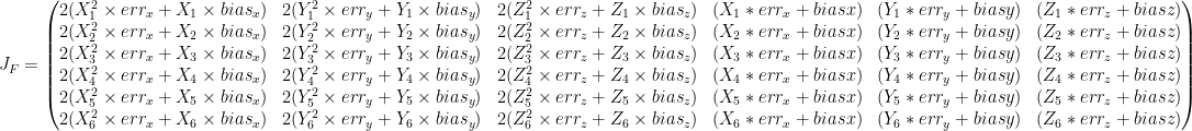

 as the unknown.
 which is “easy” to solve using a