Building Yapibot: mechanic

First version of my robot was made out of Lego mindstorm and controlled by a Raspberry Pi 1. Lego Mindstorm is amazing  and I really wish it existed when I was a kid. So I took the motors from the Lego kit and used a L293 to drive them from the Rpi.

A few hours on figuring out how to put everything together in Lego and I got the “prototype” that you can see here in action following a line using the raspberry pi camera and openCV.


Eventually, 3D printers became a thing and the price decreased. It is still a little bit expensive but it is such a nice tool that I bought a kit to build a Prusa i3 rework. It is a fork of the popular prusa I3 which is one the most popular open hardware 3D printer. I liked the idea that many part of the printer was 3D Printed and it could print itself. Kit is delivered with a good assembly instructions manual, it’s a nice building game which is not too difficult but takes a few hours.

This is it in action printing it’s first part: a cube. I could just stay for hours starring at that thing building something layer after layer … it’s some kind of magic (but much slower).


Difficult part with such 3D printer is having a good calibration. A commercial 3D printer comes already calibrated so it can be used directly out of the box but it is not the case for DIY printers. Critical part is getting the first layer correctly. As it is very close to the bed, if the extruder is too close it can touch it (it would be bad) but if it is too far away the material won’t stick and every other layers will be messy. The complete configuration and calibration process, could probably be the subject of a complete post. Anyway, after many attempts and a few customization (bed height sensor, additional cooling fan), I have now a fully armed and operational battle station 3D printer. It’s time to make the Yapibot.

There is already a lot of robot design available on 3d model sharing site but I wanted to learn as much as possible so I decided to design also the parts. I did not touch any CAD software since high school, I had to start from scratch and learn everything. I always favour open source software when available and FreeCAD was an obvious choice. It’s open source and available for linux, windows and MAC. It took me a little bit of time to sort it out, but once you get the work flow, it does the job well. Draw a 2D sketch, add the constrains (dimensions) and extrude or create a pocket. Repeat on the next face… and so on until your part is done. Many tutorials are available to get you started. As I kept the part design as simple as possible using only basic shapes it went reasonably well. Only issue I faced, other than the few bugs from time to time, has been to do modification. As the building of a part is sequential and each sketch depends on each other, sometime a small modification of a dimension on a sketch will breaks the complete part, requiring to redo the complete design.

It’s probably not the best approach but I couldn’t figure the whole thing all together so I decided to go for modularity by making a “base” where I could just screw the other parts. This makes the design of each individual part much easier and easy to replace. Good thing about having your own  3D printer is that It’s easy to redo a part if it needs to be. As I’m exclusively using  PLA as printing material (my 3D printer supports ABS but It’s not renewable, and emits toxic vapour while printing) I don’t have any remorse in trashing a part and re printing it.

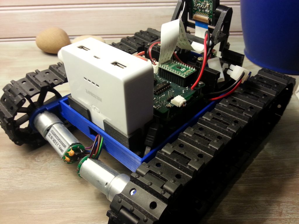
I kept to the caterpillar  because it makes the mechanics easy to design, it can run on a great variety of surface and provide a good agility to the robot. However it is not the most precise method because by design it is drifting when turning. Motors can be found here. I choose DC motors because the command electronic is simple than stepper motors. they have a low max current so two motors can be driven by a single L293D without external components or heat-sink. Finally they have built in encoder that can be used to make a closed loop control and to measure the distance moved by the robot. I choose the 1:53 gear ratio because I was a little bit concerned about the motor capabilities but 1:19 would have been better in the end. Motors are powered by a specific batteries pack made of five 1.2V 2000mA/h AAA elements.

Tracks are from makeblock: http://www.makeblock.com/track-with-track-axle-40-pack (I used one and half pack). That’s the only mechanical part not printed. Printed parts are unfortunately too slippery for this usage.

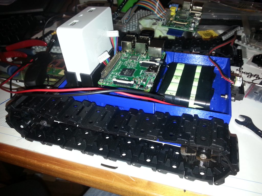
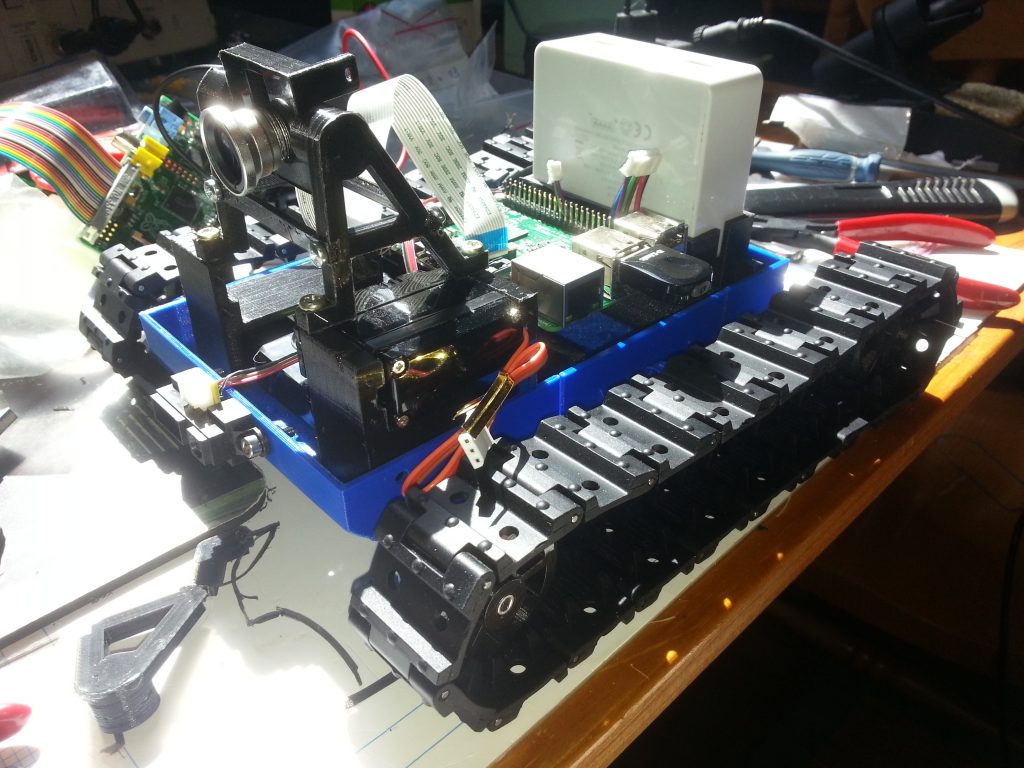
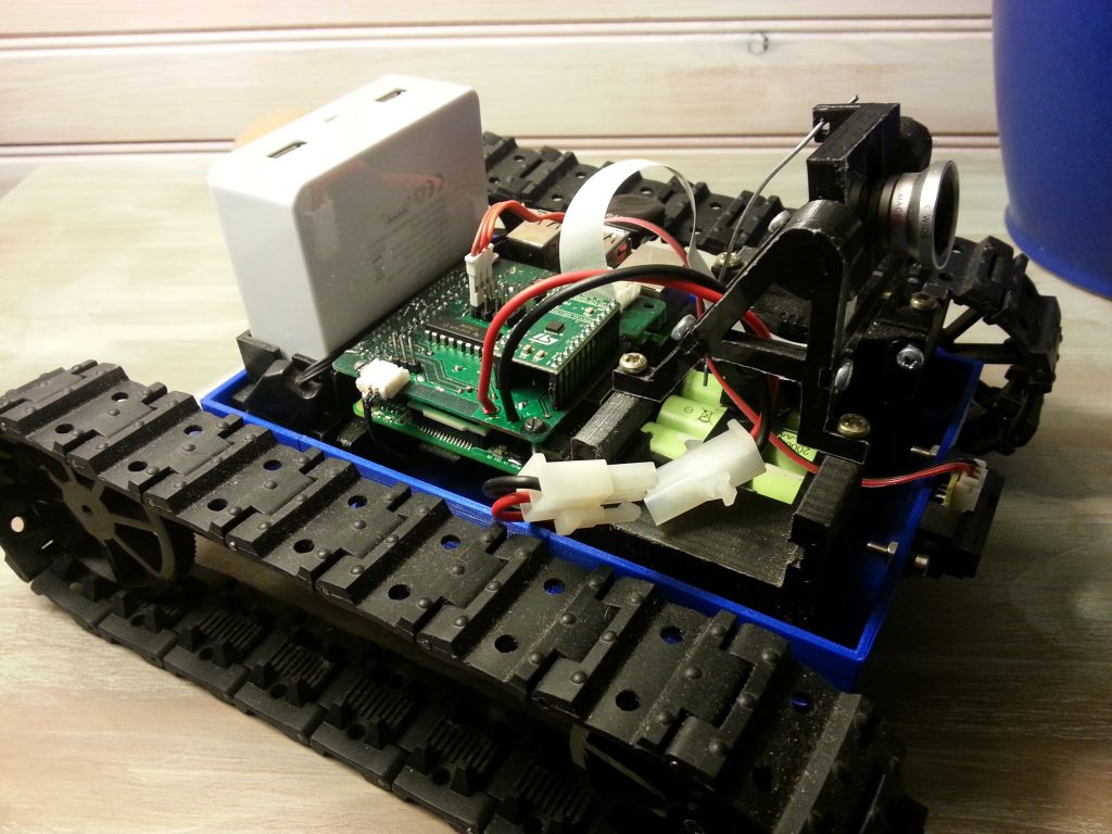
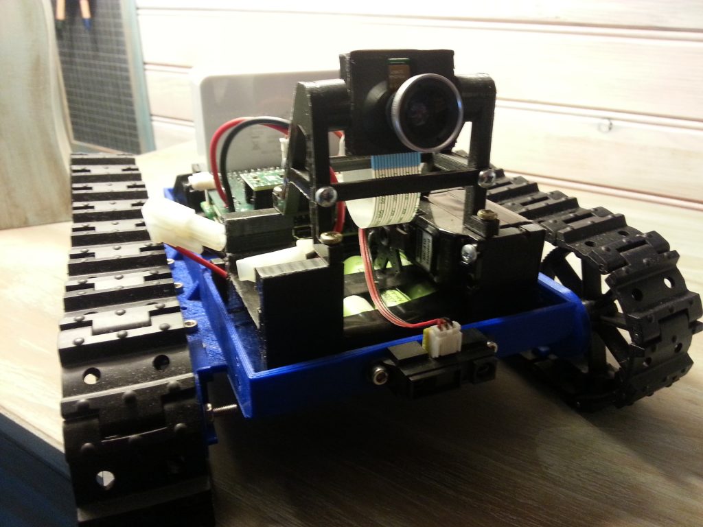
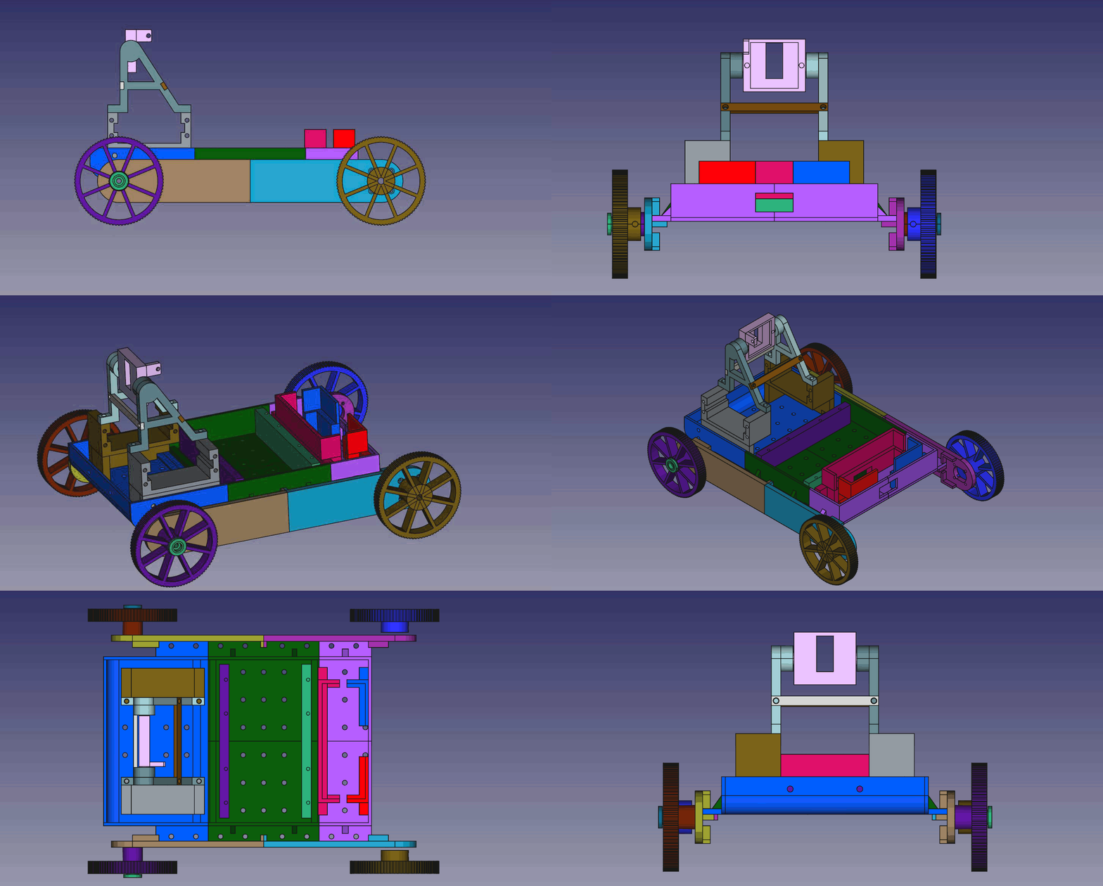
Here is the CAD result showing only the printed part.

And here are the files :FreeCAD Files.

Printing a part can takes several hours depending on the number of layers.

Work in progress ….


… and done (for the moment).


There is still an issue that I didn’t tackled yet. Motors fixing is not rigid enough and flex too much due to the motor weight and caterpillar tension. It’s not a big issue for the moment, but it might be if more precision is needed.

Building a generic active class with c++11

If you already had a look at the YapiBot source code and are familiar with multi-threaded application, you probably noticed that while the code is thread safe, I did not take any care to enforce in which context function call is made. For example, when receiving a message on the command socket, all the action resulting from this message will be done in the context of the socket thread. It’s not a big deal here because the project is still small but that might be an issue for bigger projects as it might be dangerous and may cause deadlocks. It is also difficult to control the priority of execution and might be an issue in projects having tight real time constrains.
A common design pattern to enforce the context of execution is the Active class. It’s a class which has its own execution thread and every action is going to executed in that context.

We usually differentiate two kind of method invocation to an active class.
Asynchronous call: They are fire & forget calls. Caller has no information on when the call is completed. That implies that it is not possible to have a return value.
Synchronous call: Caller needs to get a notification that the call is complete. A return value is possible but not mandatory.

A third method is also sometimes possible and somewhere in the middle: Call is asynchronous until we need to get the returned value then it waits until the value is available.

There is many active class implementation available but It was a very good exercise for me to have a looks at the possibilities of C++11 in particular the thread support functionalities. My design goal will be, by using as many as possible c++11 feature to build a base class which can be inherited from with the fewer code possible. It also needs to be as seamless as possible for the caller.

I’m going to present several steps going more and more generic which will allows me to introduce the concepts. If you are familiar with C++11 and Actives class you can just jump to the step 3 to check the result. Source code is available at the end of the post.

Step 1: Basic deferred call

#include <iostream>
#include <future>
#include <thread>
#include <chrono>

class CActiveClass
{
public:
	CActiveClass () {};
	~CActiveClass () {};

private:
	void privAsyncMethod (void) {
	        std::this_thread::sleep_for(std::chrono::seconds(2));
		std::thread::id this_id = std::this_thread::get_id();
		std::cout << "privAsyncMethod called in " << this_id << " context\n";	
	}
	int privSyncMethod (void) {
		std::this_thread::sleep_for(std::chrono::seconds(1));
		std::thread::id this_id = std::this_thread::get_id();
		std::cout << "privSyncMethod called in " << this_id << " context\n";	
		return 42;
	}
public:
	void pubAsyncMethod (void) {	
		std::async(std::launch::async, std::bind (&CActiveClass::privAsyncMethod, this));
	}
	int pubSyncMethod (void) {
		auto ret = std::async(std::launch::async, std::bind (&CActiveClass::privSyncMethod, this));
		return ret.get();
	}
};

int main ()
{
	std::thread::id this_id = std::this_thread::get_id();
	std::cout << "Main running in " << this_id << " context\n";
	CActiveClass active;
	std::cout << "calling async method from main\n";
	active.pubAsyncMethod();
	std::cout << "calling sync method from main\n";
	int ret = active.pubSyncMethod ();
	std::cout << "Synccall returned " << ret << "\n";
        return 0;
}

Our class has a public interface but all the real work is done inside the private methods. To go from one context to another we use here std::async which will launch a thread to execute the function passed as the argument. As the function is a class method we have to used std::bind which is a kind of a magic function which allows us to “package” our instance with the method call (we will see later that it can be used to bind call argument too).
The return value of std::async is an std::future which is a very nice new feature of c++11. A std::future is a value which may not be yet available. It is associated with a std::promise where the value will be posted when it is ready. You can see it as a single usage mailbox. So it is possible to get a future from a function call even if the result is not computed yet and keep going until we need to use it. Then get() will return the value, or block until it is ready. On the other side, the result is simply posted to the associated std::promise when it is available. That’s a very easy way to synchronise two threads while taking the full advantage of a distributed or multi CPU system.

So is that it ? Unfortunately no, even if our function call are deferred to another thread, it is not our class own thread and we have no way to control in which thread the execution will take place. In fact the execution can be deferred to any thread from a pool. So clearly that’s not an active class as we want it.

Also, running this give the following output:

>lythaniel@lythaniel-VirtualBox:~/ActiveClass/build$ ./ActiveClass
>Main running in 3073943296 context
>calling async method from main
>privAsyncMethod called in 3073936192 context
>calling sync method from main
>privSyncMethod called in 3073936192 context
>Synccall returned 42

In the case of the synchronous call, the output is as expected but for the asynchronous call it is not. As the privAsyncMethod takes a long time to run we shall be calling pubSyncMethod before the async call is complete. In fact, there is small pitfall here while using std::async. This function returns a future even if you don’t use it. And this future is a little bit special because it will wait for the promise to be posted when the destructor is called. Even if it is not visible in the code, this future still exists and is deleted right after the std::async invocation turning our async function into a synchronous one.

Step 2: Controling the execution context.

We saw that using std::async as a way to defer our execution to another thread was not a practical solution in this case. So we will have to spawn our own thread and use it to execute the task. Basic principle is, caller push the job into a fifo, it wakes up the processThread which in return fetchs the job from the fifo and executes it in the correct context, eventually, the result needs to be passed back to the caller. Sounds easy, but it faces an issue: every method may have a different return and argument type so it is difficult to store them and to execute them without having the knowledge of the function. That’s why the job will be packed into an polymorphic class. A pure abstract base class will only have a pure virtual execute method and we will have a class for each of the method type to call. Of course using template we won’t need to write one for each method . Fifo will store pointers to base class and the process thread just has to execute them without worrying about what’s going on behind.

class CTaskBase {
public:
        virtual void execute (void) = 0;
};

template <class C, class Ret>
class CTask : public CTaskBase
{
public:
	typedef Ret (C::*Method)(void);

	CTask (C* ptr,Method method) :
	m_Task(std::bind(method, ptr))
	{
	}

	~CTask () {}

	std::future<Ret>  get_future (void)
	{
		return m_Task.get_future();
	}

	virtual void execute (void)
	{
		m_Task();
	}

private :
	std::packaged_task< Ret (void)> m_Task;
};

To store the function call, we will use another neat feature of C++11: std::packaged_task. Push a function in it with arguments if needed (using std::bind), call it later and get the result via a future. That’s nearly all we need here but as packaged_task is specialized for a type, we still need to have an abstraction.

void CActiveclass::taskLoop (void) {
		CTaskBase * task = NULL;
		
		std::thread::id this_id = std::this_thread::get_id();
		std::cout << "CActiveClass processLoop started in " << this_id << " context\n";
		while (m_Delete.load() == false)
		{
			std::unique_lock<std::mutex> uniqueLock(m_CondMutex);
    			m_Cond.wait(uniqueLock, [this]{return m_TaskInQueue.load();});
			uniqueLock.unlock();
			
			do {

				m_TaskQueueMtx.lock();		
				if (!m_TaskQueue.empty())
				{
					task = m_TaskQueue.front();
					m_TaskQueue.pop();
				}
				else
				{
					task = NULL;
					m_TaskInQueue.store(false);
				}
				m_TaskQueueMtx.unlock();
				if (task != NULL)
				{
					task->execute ();
					delete task;
				}
			} while (task != NULL);
		}		
	}

I used a std::condition_variable as the wake up source for the task which is a little bit of overkill in that case as a semaphore could have done the job just as well, but it is a way to show it’s usage and it might be usefull if we want to add additionnal wake up source later.

Our public method now look like this:

int pubSyncMethod (void) {
		CTask<CActiveClass, int> * task = new CTask<CActiveClass, int> (this,&CActiveClass::privSyncMethod);
		auto ret = task->get_future();
		{
			std::lock_guard<std::mutex> lg (m_TaskQueueMtx);
			m_TaskQueue.push(task);
		}	
		{
			std::lock_guard<std::mutex> lg (m_CondMutex);
			m_TaskInQueue.store(true);
			m_Cond.notify_one();
		}
		return ret.get();
	}
void pubAsyncMethod (void) {
		CTask<CActiveClass> * task = new CTask<CActiveClass> (this,&CActiveClass::privAsyncMethod);
		{
			std::lock_guard<std::mutex> lg (m_TaskQueueMtx);
			m_TaskQueue.push(task);
		}	
		{
			std::lock_guard<std::mutex> lg (m_CondMutex);
			m_TaskInQueue.store(true);
			m_Cond.notify_one();
		}
	}

Runing the application we get:

>lythaniel@lythaniel-VirtualBox:~/ActiveClass/build$ ./ActiveClass
>Main running in 3074123520 context
>calling async method from main
>calling sync method from main
>CActiveClass processLoop started in 3074116416 context
>privAsyncMethod called in 3074116416 context
>privSyncMethod called in 3074116416 context
>Synctask returned 42

As expected, calling the async method is not blocking anymore and all the private method are called into the correct context.

Step 3: Making it generic.

So now that the basic is working, we have to make it generic. Remember, we want to be able to easly create any active class by just inheriting from the base class and to add our own method with a minimum of code.
Templates are going to be a great help here because they will remove the need to add code for every type of method but prior to c++11, you needed to write a template for every number of argument you needed. So you had to limit the maximum number of arguments possible and then write a template for each. Not a big deal but kind of dull work when you need to support a great number of argument. Hopefully, c++11 brings a new feature: variadic templates. Just like variadic arguments which handle “any number of arguments”, variadic template means “any number of argument types” (which can be none). it looks like this:

template <typename... Args>
void foobar (Args... args) {}

Ctask is modified accordingly and two function AsyncWrapper and SyncWrapper has been added to create them and push them into the task queue. A new wrapper is also available which return a future instead of the value itself so we can have the possibility to start a task and use the result later.

You can see  that i’m now using std::bind to bind the class instance and the method together but also the arguments.

#include <iostream>
#include <future>
#include <thread>
#include <chrono>
#include <mutex>
#include <condition_variable>
#include <queue>
#include <cassert>

template <class C>
class CActiveClass
{
public:
	CActiveClass () :
	m_Delete (false), //Order is important.
	m_TaskThread(std::bind(&CActiveClass::taskLoop, this)) {}

	~CActiveClass () 
	{
		
		m_Delete.store (true);	
		{
			//Unblock the thread.
			std::lock_guard<std::mutex> lg (m_CondMutex);
			m_TaskInQueue.store(true);
			m_Cond.notify_one();
		}
		//Wait for the thread to finish	
		m_TaskThread.join();
		//Assert in case the call queue is not empty.	
		assert (m_TaskQueue.empty()) ;

	}

private:

	class CTaskBase {
	public:
		virtual void execute (void) = 0;
	};

	template <typename Ret, typename... Args>
	class CTask : public CTaskBase
	{
	public:
		typedef Ret (C::*Method)(Args...);

		CTask (C* ptr,Method method, Args... args) :
		m_Task(std::bind(method, ptr, args...))
		{
			 
		}

		~CTask () {}

		std::future<Ret>  get_future (void)
		{
			return m_Task.get_future();
		}

		virtual void execute (void)
		{
			m_Task();
		}

	private :
		std::packaged_task<Ret ()> m_Task;
	
	};
	
	void taskLoop (void) {
		CTaskBase * task = NULL;
		
		while (m_Delete.load() == false)
		{
			//Wait for task to be run.
			std::unique_lock<std::mutex> uniqueLock(m_CondMutex);
    			m_Cond.wait(uniqueLock, [this]{return m_TaskInQueue.load();});
			m_TaskInQueue.store(false);
			uniqueLock.unlock();
			
			do {
				task = NULL;
				m_TaskQueueMtx.lock();		
				if (!m_TaskQueue.empty())
				{
					task = m_TaskQueue.front();
					m_TaskQueue.pop();
				}
				m_TaskQueueMtx.unlock();
				if (task != NULL)
				{
					task->execute ();
					delete task;
				}
			} while (task != NULL);
		}
	}

protected:
	
	template <typename... Args>
	void AsyncWrapper (C* pMe, void (C::*method)(Args...), Args... args)
	{
		assert (!m_Delete.load());			
		CTask< void, Args...> * task = new CTask< void, Args...> (pMe, method, args...);	
		{
			std::lock_guard<std::mutex> lg (m_TaskQueueMtx);
			m_TaskQueue.push(task);
		}
		
		{
			std::lock_guard<std::mutex> lg (m_CondMutex);
			m_TaskInQueue.store(true);
			m_Cond.notify_one();
		}
	}
	template <typename Ret, typename... Args>
	Ret SyncWrapper (C* pMe, Ret (C::*method)(Args...), Args... args) {
		assert (!m_Delete.load()); 
		CTask<Ret, Args...> * task = new CTask< Ret, Args...> (pMe, method, args...);
		auto ret = task->get_future();
		{
			
			std::lock_guard<std::mutex> lg (m_TaskQueueMtx); //Lock is released when lg is destroyed
			m_TaskQueue.push(task);
		}
		
		{
			std::lock_guard<std::mutex> lg (m_CondMutex); //Lock is released when lg is destroyed
			m_TaskInQueue.store(true);
			m_Cond.notify_one();
		}
	
		return ret.get();
	}
	template <typename Ret, typename... Args>
	std::future<Ret> FutureWrapper (C* pMe, Ret (C::*method)(Args...), Args... args) {
		assert (!m_Delete.load()); 
		CTask<Ret, Args...> * task = new CTask< Ret, Args...> (pMe, method, args...);
		std::future<Ret> ret = task->get_future();
		{
			
			std::lock_guard<std::mutex> lg (m_TaskQueueMtx); //Lock is released when lg is destroyed
			m_TaskQueue.push(task);
		}
		
		{
			std::lock_guard<std::mutex> lg (m_CondMutex); //Lock is released when lg is destroyed
			m_TaskInQueue.store(true);
			m_Cond.notify_one();
		}
	
		return ret;
	}

private:
	std::atomic<bool> m_Delete; //Order is important.

	typedef std::queue <CTaskBase> taskQueue_t;
	taskQueue_t m_TaskQueue;
	std::mutex m_TaskQueueMtx; //stl is not thread safe, we need to protect the queue.

	std::atomic<bool> m_TaskInQueue; //A little bit overkill for a boolean which is likely already atomic.

	std::thread m_TaskThread;

	std::mutex m_CondMutex;
	std::condition_variable m_Cond;
	
};

Using this base class to build an Active class can then easly be done.

#include "ActiveClass.h"


class CMyActiveClass : public CActiveClass<CMyActiveClass>
{
public:
	CMyActiveClass() {};
	~CMyActiveClass() {};

	int syncMultiply (int a, int b)
	{
		return SyncWrapper<int, int, int>(this, &CMyActiveClass::privMultiply, a, b);
	}
	void asyncSayHello (void)
	{
		AsyncWrapper<>(this, &CMyActiveClass::privSayHello);
	}
	std::future<float> futureDivide (float x, float y)
	{
		return FutureWrapper<float, float, float>(this, &CMyActiveClass::privDivide, x, y);
	}
private:
	int privMultiply (int a, int b)
	{
		return a * b;
	}
	void privSayHello (void)
	{
		std::cout << "Hello world !\n";
	}
	float privDivide (float x, float y)
	{
		std::this_thread::sleep_for(std::chrono::milliseconds(1000)); //That's a very long operation ...
		return x/y;
	}
};

Conclusion:
The active class presented here “do the job” but could use some improvement. constructor & destructor are potentially dangerous as the base class will be constructed before and destroyed after the herited class. This means that the task loop will be running while the herited class does not exist which can be an issue. Also I beleive that it could be improved by adding a notion of priority of the task, maybe based on the caller thread priority (for RT systems).
This was however a great show case of the possibility of c++11 and I was surprised & pleased to see how it made the building of such class easy and portable.

Source code under MIT licence: ActiveClass.tar
Sensor calibration, matrix and Newton…

In my previous post about AMHR filter I told you that the filter was taking care of the sensors error by being robust to linearity and bias error of our LSM9DS1 chip. Indeed, the Madgwick’s filter is robust against them, but minoring theses error can still be usefull because it will take less time at startup to converge to the correct orientation and it will help getting a more accurate estimation of the speed and the position of the robot.

Good news is that it is possible to perform a calibration to lower the error as some of them are due to factory issued and will be constant for a given chip. Bad news is that it is not possible to completely remove them because some part are temperature dependant and will be drifting over time.

Calibration involve running a certain number of measurements based on known conditions and based on the measurements, compute a correctionto be applied on sensor output. This will present the method I used to perform the accelerometer calibration but it can be used also for the magnetometer.

With a perfect accelerometer in a perfect robot mechanic standing on a perfect floor, the read out of the accelerometer should be \begin{bmatrix}x\ y\ z\\    \end{bmatrix} = \begin{bmatrix}0\ 0\ 1\end{bmatrix}

Of course in a real world, the sensor is not perfect and for each axis, it shows a linearity and a bias error.

\begin{bmatrix}    (X\times err_{x} + bias_{x})\ (Y \times err_{y} + bias_{y}) \ (Z \times err_{z} + bias_{z})\\    \end{bmatrix} = \begin{bmatrix}    0\ 0\ 1    \end{bmatrix}

where X , Y , and Z are the measurement done on the according axes, err_{x,y,z} is the scalling error and bias_{x,y,z} is the offset error.

Our goal will be to determine the 6 unknown from the previous equation.

Let’s imagine that we have a perfect rig available so we can position our robot in six perfectly known positions.  We can choose theses position so the gravity vector is aligned with each axis in both direction. During the calibration we just measure the output of the sensor for each orientation and we just have to solve this equation system:

\begin{pmatrix}    (X_{1}\times err_{x}+bias_{x}) & (Y_{1}\times err_{y}+bias_{y}) & (Z_{1}\times err_{z}+bias_{z})\\  (X_{2}\times err_{x}+bias_{x}) & (Y_{2}\times err_{y}+bias_{y}) & (Z_{2}\times err_{z}+bias_{z})\\  (X_{3}\times err_{x}+bias_{x}) & (Y_{3}\times err_{y}+bias_{y}) & (Z_{3}\times err_{z}+bias_{z})\\  (X_{4}\times err_{x}+bias_{x}) & (Y_{4}\times err_{y}+bias_{y}) & (Z_{4}\times err_{z}+bias_{z})\\  (X_{5}\times err_{x}+bias_{x}) & (Y_{5}\times err_{y}+bias_{y}) & (Z_{5}\times err_{z}+bias_{z})\\  (X_{6}\times err_{x}+bias_{x}) & (Y_{6}\times err_{y}+bias_{y}) & (Z_{6}\times err_{z}+bias_{z})\\    \end{pmatrix} = \begin{pmatrix}    0 & 0 &1 \\    0 & 0 &-1\\    0 & 1 & 0\\    0 & -1 &0\\    1 & 0 & 0\\    -1 & 0 & 0\\    \end{pmatrix}

Unfortunatly, I don’t have any calibrated rig available to do the measurement so it will make our life harder as we don’t known the direction of the gravity vector. However, whatever it’s direction, we still know that it’s norm is equal to 1g. So we can pose if the robot is standing still:

\sqrt{(X \times err_{x} + bias_{x})^{2} + (Y \times err_{y} + bias_{y})^{2} + (Z \times err_{z} + bias_{z})^{2}}=1

Which can be simplified as:

(X \times err_{x} + bias_{x})^{2} + (Y \times err_{y} + bias_{y})^{2} + (Z \times err_{z} + bias_{z})^{2} - 1 = 0

So to acheive our calibration process, we just have to find the roots of the following equation system:

\begin{pmatrix}    (X_{1} \times err_{x} + bias_{x})^{2} + (Y_{1} \times err_{y} + bias_{y})^{2} + (Z_{1} \times err_{z} + bias_{z})^{2}\\  (X_{2} \times err_{x} + bias_{x})^{2} + (Y_{2} \times err_{y} + bias_{y})^{2} + (Z_{2} \times err_{z} + bias_{z})^{2}\\  (X_{3} \times err_{x} + bias_{x})^{2} + (Y_{3} \times err_{y} + bias_{y})^{2} + (Z_{3} \times err_{z} + bias_{z})^{2}\\  (X_{4} \times err_{x} + bias_{x})^{2} + (Y_{4} \times err_{y} + bias_{y})^{2} + (Z_{4} \times err_{z} + bias_{z})^{2}\\  (X_{5} \times err_{x} + bias_{x})^{2} + (Y_{5} \times err_{y} + bias_{y})^{2} + (Z_{5} \times err_{z} + bias_{z})^{2}\\  (X_{6} \times err_{x} + bias_{x})^{2} + (Y_{6} \times err_{y} + bias_{y})^{2} + (Z_{6} \times err_{z} + bias_{z})^{2}\\    \end{pmatrix} = \begin{pmatrix}  1 \\  1 \\  1 \\  1 \\  1 \\  1 \\  \end{pmatrix}

Unfortunalty, that’s not so easy to solve because this equation system is not linear (some square unknown appear in the calculation).

That’s where Newton and his buddy Raphson come to save the day as they developped an algorithm which is going to be a great help in our case. The Newton Raphson method is a method to find an approximation of the root of a function by iteration.

The idea, is simple. Start with a value of your function  that you know is close to the solution. Calculate the derivate of the function for this point (which is the tangent line at this point) and determine when this tangent equals 0.  Then use this value as the new starting value and repeat the operation until you reach the needed precision.

NewtonIteration Ani

In other word for a single equation: x_{n+1} = x_{n}  - \frac{f(x_n)}{f'(x_n)}

This method can be extended to solve system of non linear equation but it gets a little bit more complex. In that case instead of dividing by f'(x) it can be shown that F(x) can be  left multiply by the inverse of its jacobian matrix.

X_{n+1} = X_{n} - J_{F}^{-1}(X_n) \times F(X_n)

A jacobian matrix is a matrix containing the first order partial derivates for each of our function.

J\begin{pmatrix}    f_0(x_0 \; x_1 \cdots x_j) \\    f_1(x_0 \; x_1 \cdots x_j) \\    \vdots \\    f_i(x_0 \; x_1 \cdots x_j) \\    \end{pmatrix}    =    \begin{pmatrix}    \frac{\partial f_0}{\partial x_0} & \frac{\partial f_0}{\partial x_1} & \cdots & \frac{\partial f_0}{\partial x_j} \\    \frac{\partial f_1}{\partial x_0} & \frac{\partial f_1}{\partial x_1} & \cdots & \frac{\partial f_1}{\partial x_j} \\    \vdots & \vdots & \ddots & \vdots\\    \frac{\partial f_i}{\partial x_0} & \frac{\partial f_i}{\partial x_1} & \cdots & \frac{\partial f_i}{\partial x_j} \\    \end{pmatrix}

So we only have to perform the partial derivate of  (X \times err_{x} + bias_{x})^{2} + (Y \times err_{y} + bias_{y})^{2} + (Z \times err_{z} + bias_{z})^{2} -1 = 0

On err _{x}, err _{y}, err _{z}, bias_{x}, bias_{y}, and bias_{z}.

The process of calculating a partial derivate is easy. Derivate according to one unknown and treat the other as constant. For example if we want to calculate the partial derivate of f_0 on err_{x}  we get:
\frac{\partial f_0}{\partial err_x} = (X_{1} \times err_{x} + bias_{x})^{2} + (Y_{1} \times err_{y} + bias_{y})^{2} + (Z_{1} \times err_{z} + bias_{z})^{2} - 1) . \partial err_x

\frac{\partial f_0}{\partial err_x} = ((X_{1} \times err_{x} + bias_{x})^{2} + C) .\partial err_x

\frac{\partial f_0}{\partial err_x} = ((X_{1} \times err_{x} + bias_{x})^{2} ) .\partial err_x

\frac{\partial f_0}{\partial err_x} =  2 (X_{1}^{2} \times err_{x} + X_{1} \times err_x)

The same way we can show that
\frac{\partial f_0}{\partial bias_x} = 2 (X_{1} * err_{x} + bias {x})

We can extrapolate our jacobian matrix for our functions:

J_F = \begin{pmatrix}    2 (X_{1}^{2} \times err_{x} + X_{1} \times bias_{x}) & 2 (Y_{1}^{2} \times err_{y} + Y_{1} \times bias_{y}) &  2 (Z_{1}^{2} \times err_{z} + Z_{1} \times bias_{z}) & (X_{1} * err_{x} + bias {x}) & (Y_{1} * err_{y} + bias {y}) & (Z_{1} * err_{z} + bias {z}) \\    2 (X_{2}^{2} \times err_{x} + X_{2} \times bias_{x}) & 2 (Y_{2}^{2} \times err_{y} + Y_{2} \times bias_{y}) &  2 (Z_{2}^{2} \times err_{z} + Z_{2} \times bias_{z}) & (X_{2} * err_{x} + bias {x}) & (Y_{2} * err_{y} + bias {y}) & (Z_{2} * err_{z} + bias {z}) \\    2 (X_{3}^{2} \times err_{x} + X_{3} \times bias_{x}) & 2 (Y_{3}^{2} \times err_{y} + Y_{3} \times bias_{y}) &  2 (Z_{3}^{2} \times err_{z} + Z_{3} \times bias_{z}) & (X_{3} * err_{x} + bias {x}) & (Y_{3} * err_{y} + bias {y}) & (Z_{3} * err_{z} + bias {z}) \\    2 (X_{4}^{2} \times err_{x} + X_{4} \times bias_{x}) & 2 (Y_{4}^{2} \times err_{y} + Y_{4} \times bias_{y}) &  2 (Z_{4}^{2} \times err_{z} + Z_{4} \times bias_{z}) & (X_{4} * err_{x} + bias {x}) & (Y_{4} * err_{y} + bias {y}) & (Z_{4} * err_{z} + bias {z}) \\    2 (X_{5}^{2} \times err_{x} + X_{5} \times bias_{x}) & 2 (Y_{5}^{2} \times err_{y} + Y_{5} \times bias_{y}) &  2 (Z_{5}^{2} \times err_{z} + Z_{5} \times bias_{z}) & (X_{5} * err_{x} + bias {x}) & (Y_{5} * err_{y} + bias {y}) & (Z_{5} * err_{z} + bias {z}) \\    2 (X_{6}^{2} \times err_{x} + X_{6} \times bias_{x}) & 2 (Y_{6}^{2} \times err_{y} + Y_{6} \times bias_{y}) &  2 (Z_{6}^{2} \times err_{z} + Z_{6} \times bias_{z}) & (X_{6} * err_{x} + bias {x}) & (Y_{6} * err_{y} + bias {y}) & (Z_{6} * err_{z} + bias {z}) \\    \end{pmatrix}

That’s a big matrix, but at the end, it is only the two same easy computation repeated each 3 times.

However we are not done yet, as Newton algorithm asks us to invert this matrix but it can be very time consuming to do so. So we can change this:
X_{n+1} = X_{n} - J_{F}^{-1}(X_n) \times F(X_n)
to look like this:
J_F(X_n)(X_{n+1} - X_n) = -F(X_n)
And solve this equation system with (X_{n+1} - X_n) as the unknown.

This time this system is linear and you may have notice that it is in the form of B = A . X which is “easy” to solve using a LU decomposition.

Fortunatly for us, we won’t have to do it ourself (that’s way too many math already! ) as a nice library called Eigen is offering to do the job for us. This library is completly template based so we just have to include the header in our code and solving this equation is as simple as:

MatrixXd Xd = jacobian.lu().solve(-F);

And we are done ! We just have to repeat the process until we reach the precision we want.

So finally how is the code looking ? very simple compared to the rest of this article 🙂

double CSensorCalibration::partialDerivateOffset (double val, double offset, double scale)
{
	double ret =  2.0 * (val * scale + offset);
	return ret;
}

double CSensorCalibration::partialDerivateScale (double val, double offset, double scale)
{
	double ret =  2.0 * (val * val * scale + val * offset);
	return ret;
}

MatrixXd CSensorCalibration::solve (MatrixXd & Meas)
{
	MatrixXd jacobian(6,6);
	MatrixXd X(6,1);
	MatrixXd F(6,1);
	int32_t iter;
        
	//Init solution
	X << 0.0, 0.0, 0.0, 1.0, 1.0, 1.0;

	for (iter = 0; iter < MAX_ITERATION; iter++)
	{
		//Calculate jacobian matrix   
		for (int i = 0; i < 6; i++)
		{
			for (int k = 0; k < 3; k++)
			{
				jacobian(i,k) = partialDerivateOffset(Meas(i,k),X(k,0),X(3+k,0));
				jacobian(i,3+k) = partialDerivateScale(Meas(i,k),X(k,0),X(3+k,0));
			}
		}
		//Compute "result" matrix.
		for (int i = 0; i < 6; i++)
		{
			F(i,0) = pow(Meas(i,0)*X(3,0) + X(0,0), 2) + pow(Meas(i,1)*X(4,0) + X(1,0), 2) + pow(Meas(i,2)*X(5,0) + X(2,0), 2) - 1;
		}

		//Check if we reached our precision requierement.
                if (abs(F.sum()) <= LIMIT_CONV_FUNCT)
		{
			break;
		}

		//Solve J_F(x_n)(x_{n+1} - x_n) = -F(x_n)
		MatrixXd Xd = jacobian.lu().solve(-F);

		//Check if we reached our precision requierement.
		if (abs(Xd.sum()) <= LIMIT_CONV_ROOT)
		{
			break;
		}

		//Update our result as the equation is giving us the (x_{n+1} - x_n).
		X = X + Xd;
	}
	return X;

}

LSM9DS1, Madgwick’s AHR filter and robot orientation

My original plan was to do several posts about general information and then go deeper into some topics, but as I’m currently working on getting the ST iNEMO LSM9DS1 intertial module to work, I thought that I might as well start this blog on this subject.

One of the thing I would like to achieve with this robot is to get it as close as possible of being capable of navigating and avoiding obstacles autonomously so it can, for example, returns to its starting position by itself.

As it will be used mostly indoor, using a GPS for precise positioning is not possible, so we have to rely on less accurate sensors. A 9DOF inertial module in the form of a LSM9DS1 from ST(datasheet), will be the main sensors to evaluate the robot position. This chip is in reality two components into a single package with a 3D accelerometer / gyroscope on one side, and a 3D magnetometer (compass) on the other side.

This kind of sensors are cheap, and are able to give the acceleration, the angular speed, as well as measuring the magnetic field but they are also not very accurate. For instance, apart from the usual “noise” of the measurement, gyroscope has an output drift which is dependant of the chip temperature and the magnetometer is subject to several measurement impairment due to the presence of other magnetic components (especially in a robot were motors are close !!!).  It is possible to  mitigate some of the errors  by performing a sensor calibration without completely removing them. Also if we want to be able to evaluate the speed and position of the robot based on the accelerometer, we need to remove the acceleration due to the gravity which means we need to be able to evaluate precisly the direction of the gravity in the sensor reference frame.

That’s where the filter proposed by Sebastian Madgwick comes into play (more info).  This filter combines data from the gyroscope, accelerometer and magnetometer to estimate the orientation (in the form a quaternion) of the device according to the earth reference (magnetic north and gravity). This algorithm acheive a good accuracy even if the device is subject to linear accelerations and is robust to sensors bias and drift. It is also open source and  C code is  available!

So, everything perfect, right? Not really and I have been struggling a little bit to get the correct output from the filter. Main reason for that the source code of the filter does not provide any documentation about the convention used for the input values: unit and axis orientation. So I had to dig into Sebastian Madgwick’s paper to find some info.

Units are simples. The filter needs to have the gyroscope data expressed as rad.s-1. For the acceleration and magnetic field, however, you can use any unit you like, because the values are normalized in the filter (only the vector orientation is important).

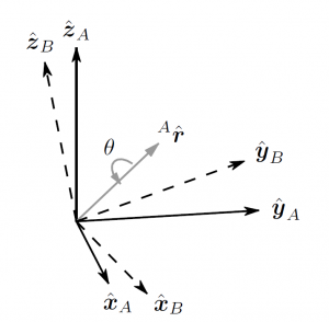
However, getting a clear answer about the axis orientation was difficult. On some discussion I found that the madgwick filter’s is using a NED  (x pointing north, y pointing east and z pointing down) convention just like in aviation.  This is not completely correct. Madgwick’s filter is indeed using a right handed axis convention but as show in Madgwick paper on page 5, the Z axis is pointing up and not down.

madgwick_axis

This can also be confirmed by the Xsens MTX user Manual  which was used to perform the algorithm evaluation and is using the same convention.

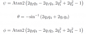
Where it gets a little bit confusing, is that Madgwick is giving the formulae to get the euler angles from the quaternion representation in his paper.

madgwick_euler_angles

Where ψ is yaw, θ is pitch and Φ is roll.

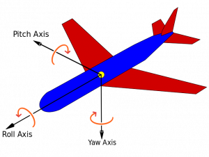
If you use theses equations, the calculated roll, pitch and yaw will be according to the aircraft convention (NED), but for the roll which need to be inverted.

Yaw_Axis_Corrected.svg

Finally, Madgwick is using variables q0, q1, q2 and q3 (or q1, q2, q3 and q4 in his paper) to represent the quaternion. But sometimes you can find quaternion represented as x, y, z and w (as in unity 3D). If for some reason, you want to use the filter output for something else, just be aware that w is equivalent to q0, not q3.

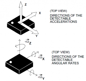
So now that we know what is expected by the filter, what about the output of the LSM9DS1 ? For accelerometer/gyroscope, the datasheet is giving the following:

LSM9DS1_accelgyro_orient

Orientation reference is left handed, so we can’t use the output as it is but swapping from left handed to right handed axis is easy, we just have to swap the X and Y axis for gyro and accelerometer.  Finally we have to align the X axis point to the front of the robot (and Y to be the left side). For Yapibot, I got lucky as the Y axis of the sensor is pointing to the front of the robot so I can just apply:

Yapibot.ax = LSM9DS1.ay
Yapibot.ay = LSM9DS1.ax
Yapibot.az = LSM9DS1.az

And for the gyro:

Yapibot.gx = LSM9DS1.gy
Yapibot.gy = LSM9DS1.gx
Yapibot.gz = LSM9DS1.gz

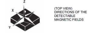
The same way, we need to adapt the ouput of the magnetometer according to our reference.

LSM9DS1_mag_orient

Be careful here because for some reason, ST did not use the same orientation of the diagram (dot on the chip is up, while for accel/gyro it is on the left) (IT’S A TRAP!). So finally, compared to the accel/gyro, only the X direction is inverted.

Yapibot.mx = LSM9DS1.my
Yapibot.my = -LSM9DS1.mx
Yapibot.mz = LSM9DS1.mz

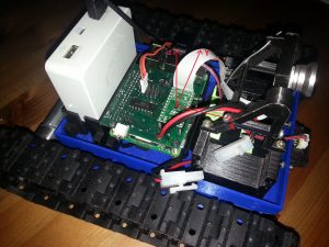
Using this convention, I have been able to correctly get the orientation of the robot.

20160820_112329

Good old time ….

So I found some videos from my robot project from when I was young and beautifull .

First one is the E=M6 cup. I’m part of the Ville d’Avray IUT team.

Second one is from the 2001 Robocup in Seattle. Unfortunatly I could not find any better video and it seems I’ve lost all my archives from that time. We are the blue team.